Inside database data files (5/3+2): Cassandra
What a Cassandra SSTable really contains: commit log, memtable, tombstones and compaction, shown with real files from a lab node.
The first three parts of this series looked at engines that edit fixed-size pages in place, or next to their old versions. Apache Cassandra takes another road, because it never edits a file. Every write ends up in a Cassandra SSTable, a sorted file that is written once and never changed. This bonus part (5/3+2 in the series numbering, after SQLite) opens a real node to show what that looks like on disk.
I don’t run Cassandra at home. Everything below comes from a one-node lab built for this post (Rocky Linux 10.2 on WSL2, Apache Cassandra 5.0.9, Temurin Java 17.0.21) and from the Apache documentation. The outputs are real: I only cut lines, and I mark each cut with [...]. With one node there is no replication, no repair and no streaming, so I say when that matters.
The Cassandra data directory
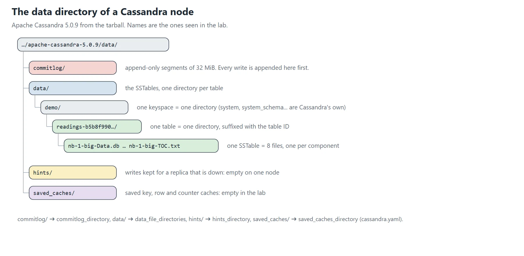
A node keeps its files in four directories. Their location comes from cassandra.yaml, and when you install from the tarball, they sit under data/.
commitlog/: the commit log, cut into segments of 32 MiB, the documented default. A fresh node already had two of them, each exactly 33,554,432 bytes.data/: the SSTables. The layout isdata/<keyspace>/<table>-<table id>/. My table landed indemo/readings-b5b8f990…. The system keyspaces (system,system_schema…) sit next to it, and they also use the same format.hints/: where writes wait for a node that is down. The reference ties it tomax_hint_window, the time during which a dead host gets hints. It stayed empty.saved_caches/: the key, row and counter caches, saved so that a restart does not start cold. Empty too.
In the previous parts, a database was a directory, but here a keyspace is a directory, and each table is a directory inside it, with a long suffix that identifies the table.
The write path: commit log, memtable, flush
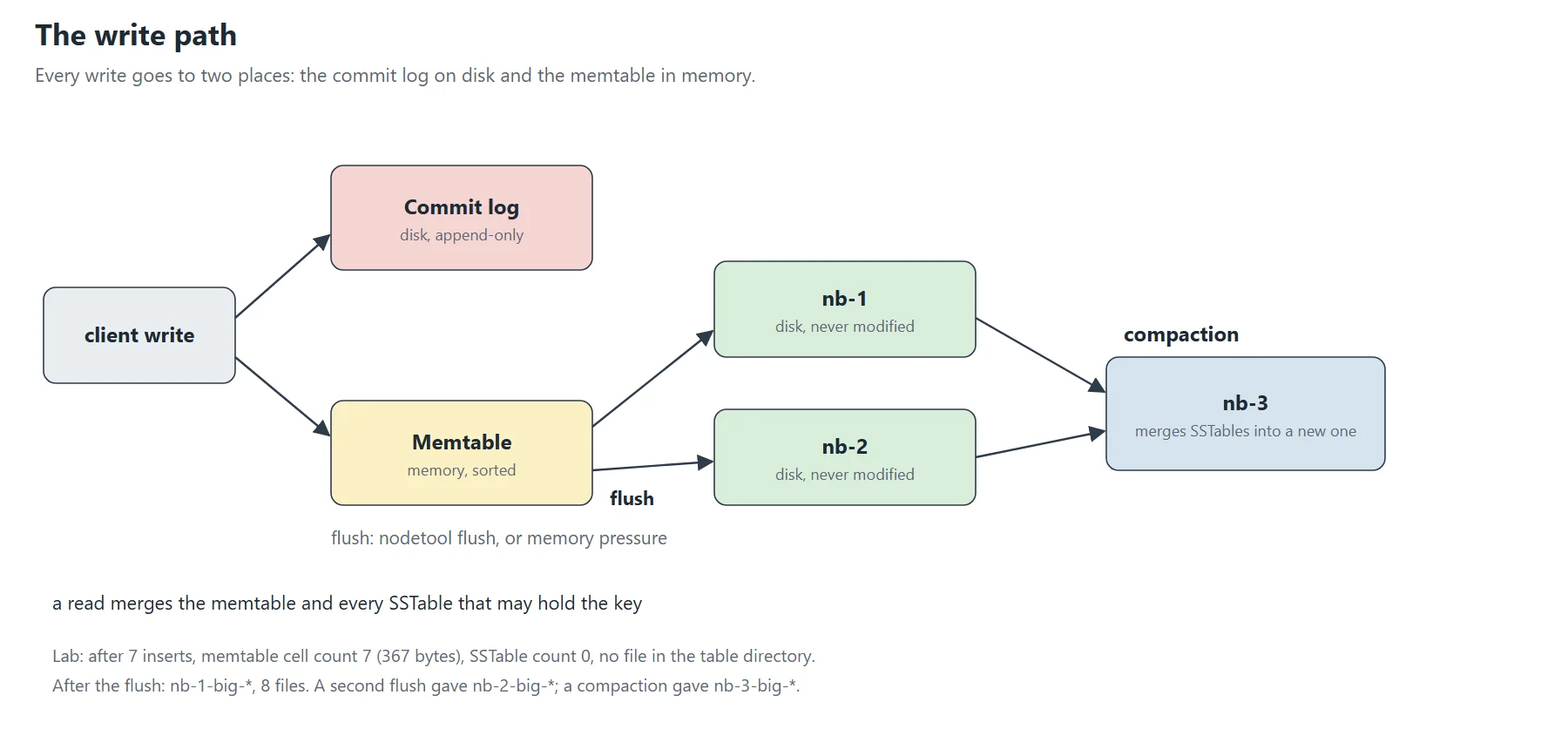
A write goes to two places. First, the commit log: Cassandra appends the change to a segment on disk, so that it survives a crash. Second, the memtable, a sorted structure in memory, usually one per table. By default the log is synced every 10 seconds (commitlog_sync: periodic, commitlog_sync_period: 10000ms), so a write is acknowledged before it is on disk. The alternative, batch, waits for the sync.
In the lab, I inserted seven rows into a new table and looked before flushing. At that point the table directory was empty, but seven cells sat in the memtable, and the commit log held their only copy on disk:
SSTable count: 0
Old SSTable count: 0
Memtable cell count: 7
Memtable data size: 367
Memtable switch count: 0
The commit log is not compressed unless you ask for it, so the keys are readable in a segment. I looked with strings:
strings CommitLog-7-*.log | grep -E "sensor-[abc]" | head -5
sensor-a
sensor-a
sensor-a
sensor-b
sensor-b
A flush turns the memtable into an SSTable. It happens when memory runs short, when the commit log nears its limit, or on demand. I ran nodetool flush demo readings and eight files appeared:
ls -l | awk '{print $5, $9}'
47 nb-1-big-CompressionInfo.db
123 nb-1-big-Data.db
10 nb-1-big-Digest.crc32
16 nb-1-big-Filter.db
36 nb-1-big-Index.db
4855 nb-1-big-Statistics.db
68 nb-1-big-Summary.db
92 nb-1-big-TOC.txt
After the flush, the two commit log segments were still there. The documentation says a segment can be deleted or recycled only once all its data is flushed to SSTables, and the segments are shared by all the tables, so I did not see one disappear.
Anatomy of a Cassandra SSTable
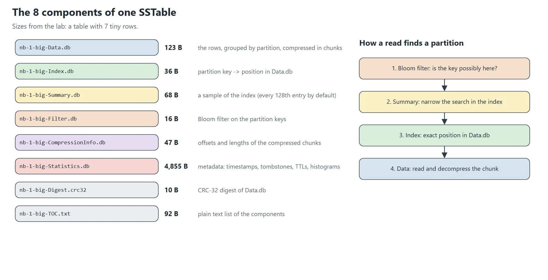
Because each file has one job, a Cassandra SSTable is a set of files that share a prefix. In the lab, nb-1-big- reads as a format version (nb), a generation number, and the format name (big, the default). The documentation does not spell this pattern out, so that is my reading of the names. It also describes a trie-based format whose index lives in Partitions.db and Rows.db instead of Index.db; I did not test it. The file TOC.txt lists the components:
cat nb-1-big-TOC.txt
CompressionInfo.db
Data.db
Digest.crc32
Filter.db
Index.db
Statistics.db
Summary.db
TOC.txt
Data.db(123 bytes): the rows, grouped by partition and compressed in chunks. The default compressor is LZ4, and the compression ratio was 0.68.Index.db(36 bytes): partition keys and their positions inData.db.Summary.db(68 bytes): a sample of the index, every 128th entry by default.Filter.db(16 bytes): the Bloom filter of the partition keys.CompressionInfo.db(47 bytes): offsets and lengths of the compressed chunks.Statistics.db(4,855 bytes): metadata such as timestamps, tombstones and TTLs. It is the biggest file here, andsstablemetadataprints histograms read from it.Digest.crc32(10 bytes): a CRC-32 digest ofData.db.
A read does not scan these files. Instead, for a partition key, Cassandra asks the Bloom filter first. A negative answer is final, while a positive one can be wrong (the table’s false-positive chance was 0.01). Then it narrows the search with the summary, finds the exact position in the index, and decompresses the chunk. After two flushes, nodetool getsstables tells which files can hold a key:
nodetool getsstables demo readings sensor-a
data/data/demo/readings-b5b8f990d6fb11f197b7370581990151/nb-1-big-Data.db
data/data/demo/readings-b5b8f990d6fb11f197b7370581990151/nb-2-big-Data.db
Partitions, rows and cells in Data.db
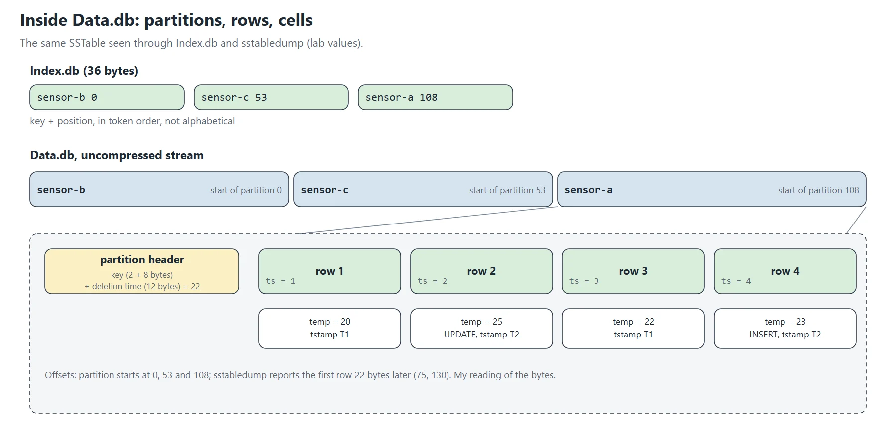
Inside Data.db, rows are grouped by partition. Partitions come in token order, the hash of the partition key, while rows inside a partition follow the clustering key. That is why my three sensors are not in alphabetical order: sensor-b comes first, then sensor-c, then sensor-a. sstabledump prints a partition like this:
sstabledump nb-1-big-Data.db
[
  {
    "partition" : {
      "key" : [ "sensor-b" ],
      "position" : 22
    },
    "rows" : [
      {
        "type" : "row",
        "position" : 22,
        "clustering" : [ 1 ],
        "liveness_info" : { "tstamp" : "2026-11-02T20:26:44.439221Z" },
        "cells" : [
          { "name" : "temp", "value" : 15 }
        ]
      },
      {
        "type" : "row",
        "position" : 37,
        "clustering" : [ 2 ],
        "liveness_info" : { "tstamp" : "2026-11-02T20:26:44.441834Z" },
        "cells" : [
          { "name" : "temp", "value" : 16 }
        ]
      }
    ]
  },
  [...]
]
Each row carries the timestamp of its INSERT in liveness_info, and each cell can also carry its own timestamp. The metadata tool confirms the token order, the compression and the absence of tombstones:
sstablemetadata nb-1-big-Data.db
Partitioner: org.apache.cassandra.dht.Murmur3Partitioner
Bloom Filter FP chance: 0.01
Compressor: org.apache.cassandra.io.compress.LZ4Compressor
Compression ratio: 0.68
First token: -2257014703785893100 (sensor-b)
Last token: 6459236691210746121 (sensor-a)
Covered clusterings: [1, 3]
Estimated droppable tombstones: 0.0
totalRows: 7
The index file is small, so I read it by hand:
xxd nb-1-big-Index.db
00000000: 0008 7365 6e73 6f72 2d62 0000 0008 7365  ..sensor-b....se
00000010: 6e73 6f72 2d63 3500 0008 7365 6e73 6f72  nsor-c5...sensor
00000020: 2d61 6c00                                -al.
Each entry is a two-byte length (0008), the key, a position and a zero, so the positions are 00, 35 and 6c: 0, 53 and 108 in the uncompressed data stream. sstabledump reports 22, 75 and 130 for the first row of each partition, which is 22 bytes after each start. That matches a header made of a two-byte key length, the eight-byte key, and a twelve-byte deletion time. The documentation does not describe the byte layout of Data.db, so treat this decoding as my reading of the output, not as a specification.
An UPDATE or a DELETE is a new write
Nothing in a Cassandra SSTable is ever edited, so to see it, I changed one value, added a row, deleted a row, deleted a whole partition, and flushed again:
UPDATE demo.readings SET temp = 25 WHERE device='sensor-a' AND ts=2;
INSERT INTO demo.readings (device, ts, temp) VALUES ('sensor-a', 4, 23);
DELETE FROM demo.readings WHERE device='sensor-b' AND ts=2;
DELETE FROM demo.readings WHERE device='sensor-c';
As a result, the second SSTable, nb-2, contains only these changes. The update is a cell with its own timestamp, and the deletes are tombstones, one for a row and one for a whole partition:
sstabledump nb-2-big-Data.db
[
  {
    "partition" : {
      "key" : [ "sensor-b" ],
      "position" : 22
    },
    "rows" : [
      {
        "type" : "row",
        "position" : 22,
        "clustering" : [ 2 ],
        "deletion_info" : { "marked_deleted" : "2026-11-02T20:27:29.783855Z", "local_delete_time" : "2026-11-02T20:27:29Z" },
        "cells" : [ ]
      }
    ]
  },
  {
    "partition" : {
      "key" : [ "sensor-c" ],
      "position" : 57,
      "deletion_info" : { "marked_deleted" : "2026-11-02T20:27:29.787731Z", "local_delete_time" : "2026-11-02T20:27:29Z" }
    },
    "rows" : [ ]
  },
  {
    "partition" : {
      "key" : [ "sensor-a" ],
      "position" : 80
    },
    "rows" : [
      {
        "type" : "row",
        "position" : 80,
        "clustering" : [ 2 ],
        "cells" : [
          { "name" : "temp", "value" : 25, "tstamp" : "2026-11-02T20:27:29.773920Z" }
        ]
      },
      {
        "type" : "row",
        "position" : 94,
        "clustering" : [ 4 ],
        "liveness_info" : { "tstamp" : "2026-11-02T20:27:29.779577Z" },
        "cells" : [
          { "name" : "temp", "value" : 23 }
        ]
      }
    ]
  }
]
The old values, 21 and 16 and the rows of sensor-c, are still in nb-1, untouched. A read then merges both files and keeps the newest answer: the SELECT returned five rows with temp = 25. The documentation puts it simply: Cassandra treats a deletion as an insertion.
Compaction rewrites the files
If left alone, SSTables pile up, and every read has to look into more of them. Compaction merges them into a new Cassandra SSTable and drops what is out of date. In the lab I disabled automatic compaction on the table, so I could run it by hand:
nodetool compact demo readings
141 nb-3-big-Data.db

nodetool compactionhistory
Compaction History:
id                                   keyspace_name columnfamily_name compacted_at            bytes_in bytes_out rows_merged compaction_properties
f61913d0-d6fb-11f1-97b7-370581990151 demo          readings          2026-11-02T21:28:28.031 213      132       {2:3}       {compaction_type:Major compaction}
After the compaction, two SSTables of 123 and 90 bytes had become one of 141 bytes. In the history, rows_merged {2:3} should mean that three partitions were found in two SSTables each (my reading). The history reports 132 bytes written while the Data.db file is 141 bytes; I did not dig into the gap. The merged file kept the update (25 replaced 21) and dropped the values covered by tombstones, but the tombstones themselves are still there:
sstabledump nb-3-big-Data.db
[
  {
    "partition" : {
      "key" : [ "sensor-b" ],
      "position" : 22
    },
    "rows" : [
      {
        "type" : "row",
        "position" : 22,
        "clustering" : [ 1 ],
        "liveness_info" : { "tstamp" : "2026-11-02T20:26:44.439221Z" },
        "cells" : [
          { "name" : "temp", "value" : 15 }
        ]
      },
      {
        "type" : "row",
        "position" : 37,
        "clustering" : [ 2 ],
        "deletion_info" : { "marked_deleted" : "2026-11-02T20:27:29.783855Z", "local_delete_time" : "2026-11-02T20:27:29Z" },
        "cells" : [ ]
      }
    ]
  },
  {
    "partition" : {
      "key" : [ "sensor-c" ],
      "position" : 74,
      "deletion_info" : { "marked_deleted" : "2026-11-02T20:27:29.787731Z", "local_delete_time" : "2026-11-02T20:27:29Z" }
    },
    "rows" : [ ]
  },
  {
    "partition" : {
      "key" : [ "sensor-a" ],
      "position" : 97
    },
    "rows" : [
      {
        "type" : "row",
        "position" : 97,
        "clustering" : [ 1 ],
        "liveness_info" : { "tstamp" : "2026-11-02T20:26:44.426582Z" },
        "cells" : [
          { "name" : "temp", "value" : 20 }
        ]
      },
      {
        "type" : "row",
        "position" : 111,
        "clustering" : [ 2 ],
        "liveness_info" : { "tstamp" : "2026-11-02T20:26:44.432537Z" },
        "cells" : [
          { "name" : "temp", "value" : 25, "tstamp" : "2026-11-02T20:27:29.773920Z" }
        ]
      },
      {
        "type" : "row",
        "position" : 130,
        "clustering" : [ 3 ],
        "liveness_info" : { "tstamp" : "2026-11-02T20:26:44.435827Z" },
        "cells" : [
          { "name" : "temp", "value" : 22 }
        ]
      },
      {
        "type" : "row",
        "position" : 145,
        "clustering" : [ 4 ],
        "liveness_info" : { "tstamp" : "2026-11-02T20:27:29.779577Z" },
        "cells" : [
          { "name" : "temp", "value" : 23 }
        ]
      }
    ]
  }
]
The default strategy is size-tiered (STCS), which is what the table used. The documentation also describes leveled (LCS), time-window (TWCS) and unified (UCS) compaction, and recommends UCS for new workloads, but I only ran STCS.
Why the files do not shrink at once
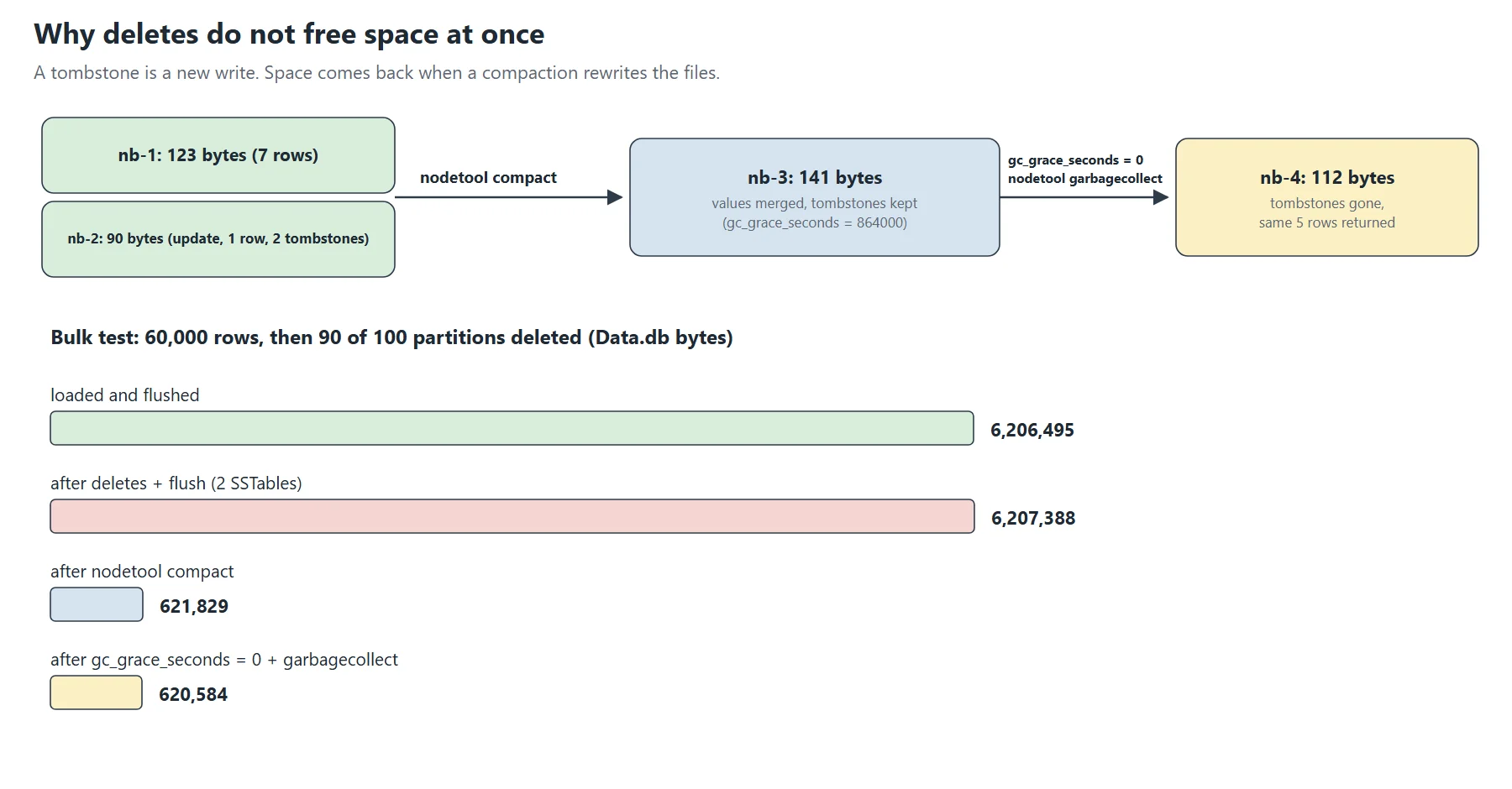
A tombstone has to outlive the data it covers, so that every replica learns about the deletion. This is the job of gc_grace_seconds, ten days by default. The documentation adds that a tombstone is removed only by a compaction after that delay, and only if all the SSTables holding older data take part in the same compaction.
To see the effect on size, I loaded 60,000 rows into a second table (100 partitions of 600 rows), deleted 90 partitions, and measured the Data.db files at each step:
| Step | Data.db bytes | SSTables |
|---|---|---|
| Loaded and flushed | 6,206,495 | 1 |
| After deleting 90 partitions and flushing | 6,207,388 | 2 |
| After nodetool compact | 621,829 | 1 |
| After gc_grace_seconds = 0 and garbagecollect | 620,584 | 1 |
The delete made the directory bigger, from 6,221,956 to 6,229,063 bytes, because tombstones are new data. Then the compaction gave the space back, and the data fell from about 6.2 MB to 0.62 MB. The last step removed 1,245 more bytes, which fits the 90 partition tombstones. I did it in the lab like this:
ALTER TABLE demo.bulk WITH gc_grace_seconds = 0;
nodetool garbagecollect demo bulk
Do not copy that on a real cluster. If a replica was down while the tombstone existed and the tombstone is purged before that replica comes back, the deleted data can reappear. The documentation calls these zombies. On one node, however, it is safe.
One detail about the tools: sstablemetadata estimates droppable tombstones with a grace period of zero unless you pass --gc_grace_seconds, so it printed 0.0136 by default, and 0.0 when I passed 864000, the real setting of the table.
Cassandra next to the three engines
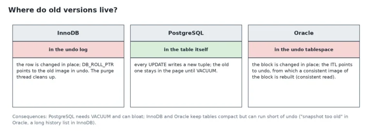
| InnoDB | PostgreSQL | Oracle | Cassandra | |
|---|---|---|---|---|
| Unit on disk | 16 KB page | 8 KB page | 8 KB block by default | an immutable Cassandra SSTable |
| UPDATE | in place, old version in undo | a new tuple version in the table | in place, before-image in undo | a new cell with a newer timestamp, in a new SSTable |
| DELETE | record marked, purged later | tuple left in place until VACUUM | row removed in the block, high water mark stays | a tombstone, a new write |
| Space comes back with | a table rebuild | VACUUM | SHRINK SPACE or MOVE | compaction, after gc_grace_seconds |
None of these choices is better in absolute terms. Cassandra pays for fast, sequential writes with background work: every update leaves an old version behind, and compaction has to clean up later. When you know that, a growing data directory after a big delete stops being a surprise.
This post is part of a series of sysadmin notes (tag “sysadmin notebook”).
Series “Inside database data files”, part 5/3+2 (bonus). · Part 3/3 and the comparison · Version française
Sources
- Apache Cassandra 5.0 documentation: storage engine (commit log, memtable, SSTable components), compaction overview (strategies, tombstones,
gc_grace_seconds) and thecassandra.yamlreference. - The lab: Rocky Linux 10.2, Apache Cassandra 5.0.9, Temurin Java 17.0.21, WSL2, one node. Tested on one node only.